Aharonov-Bohm Effect

Consider an “ideal” solenoid:

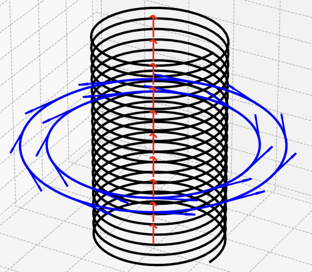
Inside the solenoid, there’s a constant magnetic field along the \(\widehat z\) direction (red arrows). Surrounding the solenoid, a vector potential exists in the \(\widehat\phi\) direction (blue arrows). However, this has no effect on a charge because magnetic field is zero outside the solenoid. In other words, even if the magnetic field inside the solenoid is incredibly strong, it’s like it doesn’t exist outside. It’s as if the magnetic field is trapped inside, not affecting anything on the outside.

This explanation originates from classical electromagnetics. But what happens in the quantum realm?

Considering the Hamiltonian that includes the Lorentz force within the solenoid:

\[\mathcal{H}=\frac{1}{2m} (\mathbf{p}-q \mathbf{A})^{2}+V\]

Here, the vector potential \(\mathbf A\) has only azimuthal component. To determine \(\mathbf A\), we can apply Ampére’s Law:

\[\oint_c \mathbf A \cdot d\vec \ell = \int_S \nabla \times \mathbf A \cdot d \vec a = \Phi\]

For the area outside the solenoid, the magnetic flux \(\Phi\) is a constant \(\Phi = \pi a^2 B\).

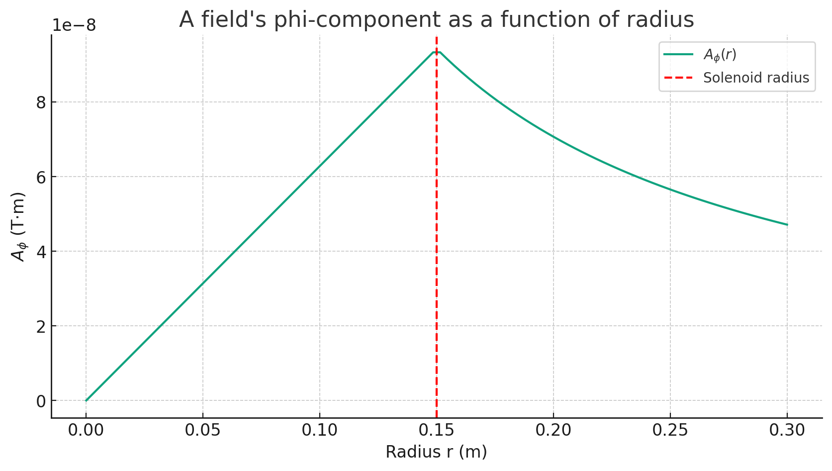
Therefore, \(\mathbf A = \frac{\Phi}{2\pi r}\hat \phi\) outside the solenoid.

While the detailed proof of this phenomenon is beyond the scope of this post, it’s essential to highlight that the vector potential \(\mathbf A\) exists outside the solenoid, even when there’s no magnetic field \(\mathbf B\). For now, let’s focus on the azimuthal component of \(\mathbf A\) (since the other components are zero), as shown in the graph below. However, remember that the full proof of these concepts isn’t the main aim here.

What matters here is focusing more on the overarching conclusions rather than getting details of the proof that follows. Next, we apply the Schrödinger equation:

\[i\hbar \frac{\partial\Psi}{\partial t} =\mathcal{H}\Psi\]

And using \(\mathbf A\), the Hamiltonian \(\mathcal{H}\) becomes:

\[\begin{aligned}\mathcal{H}&=\frac{1}{2m} (\mathbf{p}-q \mathbf{A})^{2}+V \\&=\frac{1}{2m} \left[-\hbar^2\nabla^2+q^2 A^2+2i\hbar q\mathbf A \cdot\nabla\right] \\&=\frac{1}{2m} \left[-\frac{\hbar^2}{b^2}\frac{\partial^2}{\partial \phi}+\left(\frac{q^2 \Phi^2}{2\pi b}\right)^2+i\frac{\hbar q \Phi}{\pi b^2}\frac{\partial}{\partial \phi} \right]\end{aligned}\]

Substituting into Schrödinger equation and rearranging, we get:

\[\frac{\partial^2 \psi}{\partial \phi^2}-2i\beta\frac{d\psi}{d\phi}+\epsilon\psi=0\]

where \(\beta=\frac{q\Phi}{2\pi\hbar}\) and \(\epsilon=\frac{2mE}{\hbar^2}-\beta^2\)

Let’s set \(\phi = Ae^{i\lambda \phi}\), then:

\[-\lambda^2 + 2\lambda \beta + \epsilon = 0\]

From this, we find:

\[\lambda = \beta \pm \sqrt{\beta^2 +\epsilon} = \beta \pm \frac{b}{\hbar}\sqrt{2mE}\]

Applying the boundary condition:

\[\psi(\phi) = \psi(\phi + 2\pi)\]

we determine:

\[\lambda = n \quad(0,\pm 1,\pm 2, \dots)\]

Rearranging the equation for \(E\), we get:

\[E_n = \frac{\hbar^2}{2m}\left(n-\frac{q\Phi}{2\pi\hbar}\right)\]

This calculation may have been time-consuming, but it brings us to an important point.

Let’s return to the Aharonov-Bohm Effect.

Potentials themselves are significant. In classical mechanics, the potential does not affect gauge transformation. We need to examine if the same holds in quantum mechanics.

Considering a gauge transformation:

\[\mathbf A \rightarrow \mathbf A' = \mathbf A + \nabla + \Lambda\]

the wave function transforms as:

\[\psi' = e^{iq\Lambda/\hbar}\psi\]

which might suggest \(\psi' = \psi\) when \(\Lambda = 0\)

However, actually,

\[\Lambda = \int_P \mathbf A \cdot d\mathbf r\]

In this case, with only the vector potential present outside the solenoid, if \(P\) is a closed path:

\[\Lambda = \int_C \mathbf A \cdot d\mathbf r = \Phi\]

This results in an effect on the phase of the wave function. We can infer that the vector potential has an effect. This is the essence of the Aharonov-Bohm Effect.

Email